Dynamic Programming
Dynamic programming(DP) is an algorithmic technique of recursively dividing the problem into smaller subproblems and solving the subproblems while memoizing the results to solve the original problem. If this sounds similar to divide and conquer, then you are right. The only thing that distinguishes DP from divide and conquer is the memoization of subproblems. DP approach can be applied when the following two conditions hold:
- The problem can be solved by combining the solutions to smaller subproblems.
- The subproblems overlap.
The point of DP is to memoize the overlapping subproblems so that you don’t have to solve the same subproblem multiple times, which can greatly reduce the time complexity.
DP Example
To get a sense, let’s consider a classic example of Fibonacci sequence. The $n$th Fibonacci number is defined as the following.
\[Fibo(n)= \begin{cases} 0 &\text{if }n=0\\ 1 &\text{if }n=1\\ Fibo(n-1)+Fibo(n-2) &\text{otherwise} \end{cases}\]To find the $n$th Fibonacci number, we need to add the the $(n-1)$th and the $(n-2)$th Fibonacci number. Then again, to get the $(n-1)$ Fibonacci number, we need $(n-2)$th and $(n-3)$th, for $(n-2)$th we need $(n-3)$th and $(n-4)$th, and so on. The following figure is the recursion tree for $Fibo(5)$.
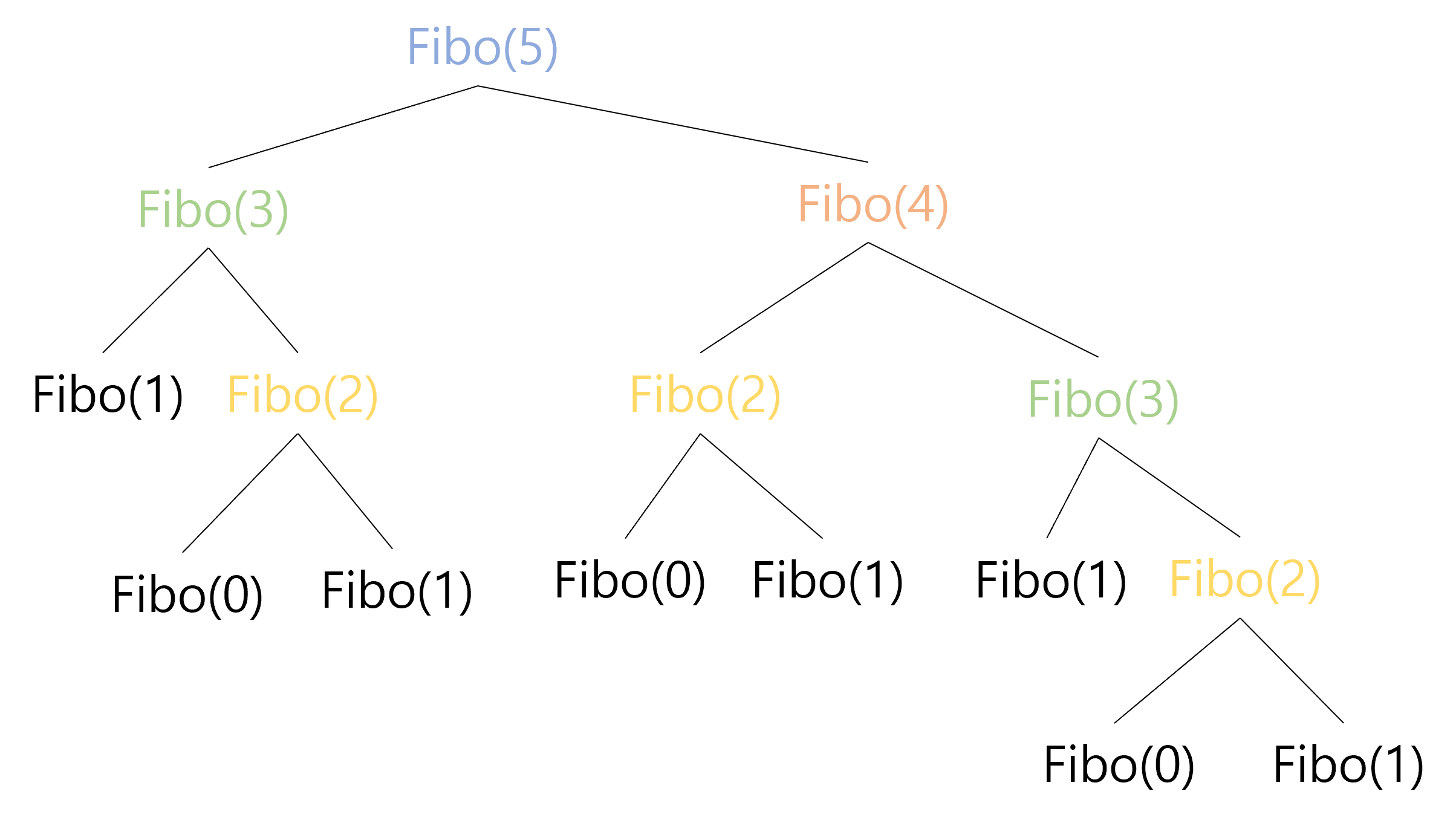
As you can observe, solving $Fibo(5)$ involves solving the same subproblems multiple times; there are 2 occurrences of $Fibo(3)$ and 3 occurrences of $Fibo(2)$ in the recursion tree. We can imagine that as as $n$ increases, we would have even more occurrences of overlapping subproblems. However, solving the subproblems from scratch - that is, expanding the whole recurence tree all the way down to the base cases - is inefficient. After all, $Fibo(k)$ for a constant $k$ is a constant integer. Therefore, once we compute $Fibo(k)$, we can memoize the corresponding constant and directly access the value without expanding the recursion everytime we need the value of $Fibo(k)$ in the future. Based on this idea, we can solve $Fibo(n)$ in $O(n)$ time by filling a 1D array, as appears in the following figure.
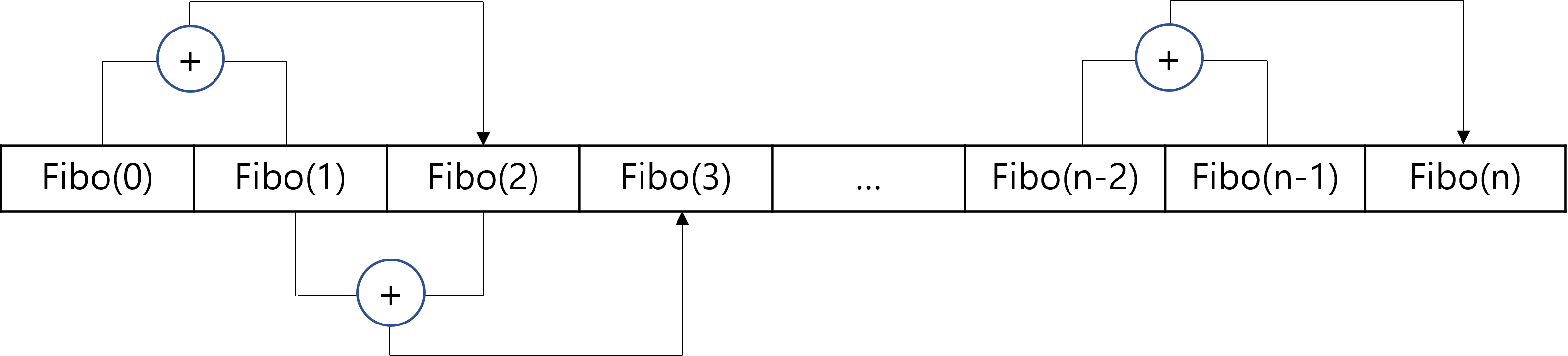
We start by filling out the first two cells which are the base cases, and then we simply add two consecutive cells to find the value for the next cell. Since we memoize the computed value in the array, we can directly access the value without recomputing it, whenever we need the value. We can simply repeat adding two cells and storing the value in the next cell until we reach the $n$th cell, which would contain the value of $Fibo(n)$.
Deriving DP from Recurrence
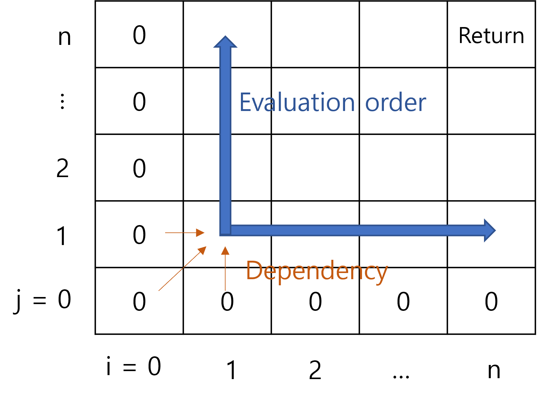
The key to writing a DP solution is finding an appropriate recurrence. Once you have a recurrence, the rest - the memoization data structure, the order of evaluation, time complexity, return value, etc - often can be easily derived. As an example, consider the following recurrence named $SomeRandomRecurrence$, abbreviated as $SRR$.
\[SRR(i, j)= \begin{cases} 0 &\text{if }i=0 \text{ or } j=0\\ SRR(i-1, j-1)+1 &\text{if } SomeRandomCondition\\ \max(SRR(i-1,j),SRR(i,j-1) )&\text{otherwise} \end{cases}\]Let’s suppose we want to return $SRR(n,n)$ at the end. Since we do not have any description of the recurrence, we don’t even know what problem we are solving. However, we can still figure out an appropriate memoization data structure and the evaluation order. Observe that $SRR(i,j)$ only depends on $SRR(i-1,j)$, $SRR(i,j-1)$, and $SRR(i-1,j-1)$. Since $SRR(n,n)$ would have no dependency on $SRR$ with indices greater than $n$, we are only interested in $SRR(i,j)$ where the parameters $i, j$ ranges from $0$ to $n$. We have $n^2$ different pairs of parameters, or in other words $n^2$ different subproblems, which means a 2D array would be appropriate as the data structure. Also, it is obvious that the evaluation order would be from lower to higher index, since we need to know the values in lower indices to find the values for higher indices.
Longest increasing Subsequence
Our very own Jeep Kaewla has created the following video explainer of the LIS problem:
Relevent LeetCode Practice (by Tristan Yang)
- LeetCode 509 — Fibonacci Number (Easy)
- Relevance: Mirrors the classic example: naive recursion for Fibonacci runs in exponential time ($\approx \Theta(\varphi^n)$ with the golden ratio $\varphi$), but with memoization or bottom-up DP it becomes linear time $O(n)$. (Also note: if we consider the size of Fibonacci numbers, computing $F(n)$ exactly involves handling $\Theta(n)$-digit integers, but here we focus on the recurrence cost.)
- ECE 374 Process: Start from the definition $F(n) = F(n-1) + F(n-2)$ with base cases $F(0)=0$, $F(1)=1$. First add memoization (store results in an array or map to avoid recomputation), then convert to an iterative bottom-up solution using two variables (for $O(1)$ space).
- Resource: LeetCode official editorial for Fibonacci.
- Takeaway: Memoization collapses an exponential recursion into linear work; converting to tabulation (bottom-up) removes recursion overhead entirely.
- LeetCode 70 — Climbing Stairs (Easy)
- Relevance: Same Fibonacci-type recurrence (each state depends on the two previous states). It’s a perfect small problem to practice three approaches: memoized recursion vs. bottom-up tabulation vs. an $O(1)$ space optimized DP.
- ECE 374 Process: Derive the recurrence $f(n) = f(n-1) + f(n-2)$ with base cases $f(0)=1$, $f(1)=1$ (if we interpret “one way” to stay at the ground step). Show a memoized $O(n)$ solution and then the equivalent iterative solution that uses two variables (previous two results) instead of an entire array.
- Resource: NeetCode explanation video.
- Takeaway: Identify the recurrence relation, then decide on memoization or table-filling. Optimize space if possible once you understand the dependency pattern.
- LeetCode 198 — House Robber (Medium)
- Relevance: Corresponds to the lecture slide’s “smart recursion” example. After defining subproblem optimal solutions, you get the recurrence: $dp[i] = \max(dp[i-1], dp[i-2] + a_i)$, where $a_i$ is the money at house $i$.
- ECE 374 Process: Define $dp[i]$ as the maximum amount that can be robbed from the first $i$ houses. You can derive the above recurrence by deciding to rob or skip the $i$-th house. Implement via memoized recursion or iteratively fill an array from $i=1$ to $n$. Finally, optimize to $O(1)$ space by only keeping the last two values ($dp[i-1]$ and $dp[i-2]$).
- Resource: NeetCode video on House Robber.
- Takeaway: Dynamic Programming = define subproblems, establish recurrence with choices, set base cases, then compute in a safe order (recursively or iteratively). Space can often be compressed given the recurrence dependencies.
Supplemental Problems
-
LeetCode 746 — Min Cost Climbing Stairs
Another Fibonacci-style 1D DP; good practice to implement with memoization and then optimize to $O(1)$-space tabulation. -
LeetCode 91 — Decode Ways
Recurrence with branching (each digit or pair of digits can form a letter if valid). A naive recursion is exponential, but memoization/DP trims it to polynomial time. -
LeetCode 322 — Coin Change
A classic unbounded coin change: define $dp[x] = 1 + \min_{c \in \text{coins}} dp[x-c]$. Perfect for comparing a top-down memo vs bottom-up implementation. -
LeetCode 518 — Coin Change II
Count the number of ways to form an amount. Order of iteration (coins-first vs. amount-first) matters to avoid double counting permutations, a good lesson in table design. -
LeetCode 62 — Unique Paths
A 2D DP with simple dependencies (each cell = sum of top and left). Good introduction to filling a table and even doing it in-place or with $O(n)$ space by reusing a single row/column. -
LeetCode 63 — Unique Paths II
Same grid DP but with obstacles. Reinforces careful handling of base cases and blocked cells (if an obstacle is present, that path count is 0). -
LeetCode 931 — Minimum Falling Path Sum
A row-by-row DP in a matrix; shows local transitions (from directly above or above-left/right) and how to do in-place updates or use a rolling array to save space. -
LeetCode 583 — Delete Operation for Two Strings
Effectively the Longest Common Subsequence (LCS) problem in disguise (minimum deletions = total length of strings - 2 * LCS length). Good practice to set up a 2D DP and relate it to a simpler 1D interpretation. -
LeetCode 139 — Word Break
A 1D DP over string prefixes; can be solved via top-down recursion with memo or bottom-up iteration checking each possible split. (Transforms an exponential brute force into $O(n^2)$.) -
LeetCode 213 — House Robber II
Like House Robber, but houses are in a circle (first and last are adjacent). Reduce it to two linear problems (rob 1..n-1, or rob 2..n) and take the max. Good practice in modeling constraints by splitting into multiple DP runs.
Additional Resources
- Textbooks
- Erickson, Jeff. Algorithms
- Skiena, Steven. The Algorithms Design Manual
- Chapter 10.1 - Caching vs. Computation
- Chapter 10.3 - Longest Increasing Subsequence
- Cormen, Thomas, et al. Algorithms (Forth Edition)
- Chapter 14 - Dynamic Programming
- Sariel’s Lecture 13
