I. Undirected graphs
Definition
An undirected (simple) graph G = (V, E) is a 2-tuple:
- V is a set of vertices (also referred to as nodes/points)
- E is a set of edges where each edge e belong to E is a set of the form {u, v} with u, v belong to V and u not equala to v.
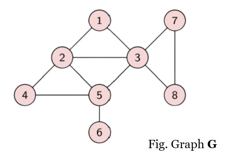
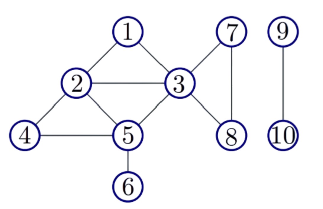
Example: In figure, G= (V,E) where V = {1,2,3,4,5,6,7,8} ; E = {(1, 2), (1, 3), (2, 3), (2, 4), (2, 5), (3, 5), (3, 7), (3, 8), (4, 5), (5, 6), (7, 8)}
Notation and Convention
An edge in an undirected graphs is an unordered pair of nodes and hence it is a set. Conventionally we use uv for {u, v} when it is clear from the context that the graph is undirected.
- u and v are the end points of an edge {u, v}
- Multi-graphs allow:
- loops which are edges with the same node appearing as both end points
- multi-edges: diferent edges between same pairs of nodes
Graph Representation I - Adjacency Matrix
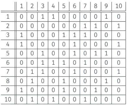
Represent G = (V, E) with n vertices and m edges using a n x n adjacency matrix A where
- A[i, j] = A[j, i] = 1 if {i, j} $\in$ E and A[i, j] = A[j, i] = 0 if {i, j} $\notin$ E.
- Advantage: can check if {i, j} $\in$ E in O(1) time
- Disadvantage: needs $\Omega$ ($n^2$) space even when m « n$^2$
Example:
|
|
|
Graph Representation II - Adjacency List
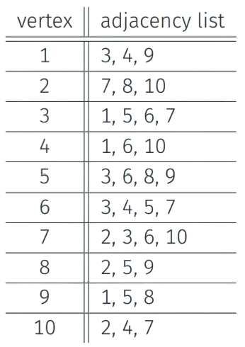
Represent G = (V, E) with n vertices and m edges using adjacency lists:
-
For each u $\in$ V, Adj(u) = {v {u, v} $\in$ E}, that is neighbors of u. Sometimes Adj(u) is the list of edges incident to u. - Advantage: space is O(m + n)
- Disadvantage: cannot “easily” determine in O(1) time whether {i, j} $\in$ E
- By sorting each list, one can achieve O(log n) time
- By hashing “appropriately”, one can achieve O(1) time.
Example:
|
|
|
|
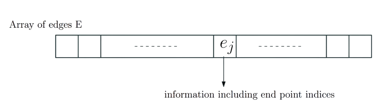
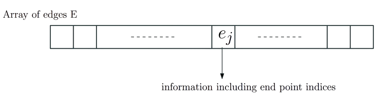
Concrete Representation
Assume vertices are numbered arbitrarily as {1, 2,…, n}.
- Edges are numbered arbitrarily as {1, 2,…, m}.
- Edges stored in an array/list of size m. E[j] is j$^{th}$ edge with info on end points which are integers in range 1 to n.
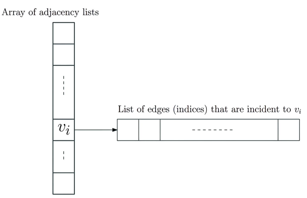
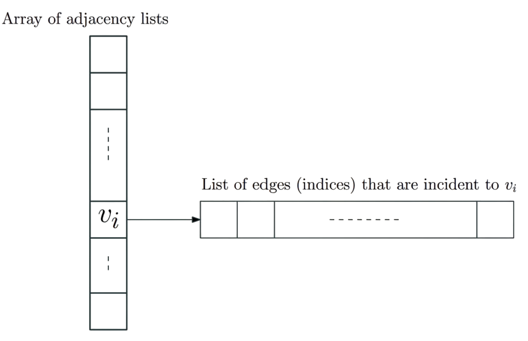
- Array Adj of size n for adjacency lists. Adj[i] points to adjacency list of vertex i. Adj[i] is a list of edge indices in range 1 to m.
|
|
- Advantages:
- Edges are explicitly represented/numbered. Scanning/processing all edges easy to do.
- Representation easily supports multigraphs including self-loops.
- Explicit numbering of vertices and edges allows use of arrays: O(1)-time operations are easy to understand.
- Can also implement via pointer based lists for certain dynamic graph settings.
Connectivity
Given a graph G = (V, E):
- path: sequence of distinct vertices $v_1$ , $v_2$ ,…, $v_k$ such that $v_i$ $v_{i+1}$ $\in$ E for 1 $\le$ i $\le$ k-1. The length of the path is k-1 (the number of edges in the path) and the path is from v$_1$ to v$_k$. Note: a single vertex u is a path of length 0.
- cycle: sequence of distinct vertices $v_1$, $v_2$,…, $v_k$ such that {$v_i$, $v_{i+1}$} $\in$ E for 1 $\le$ i $\le$ k1 and {$v_1$, $v_k$} $\in$ E. Single vertex not a cycle according to this defnition.
- Caveat: Some times people use the term cycle to also allow vertices to be repeated; we will use the term tour.
- A vertex u is connected to v if there is a path from u to v.
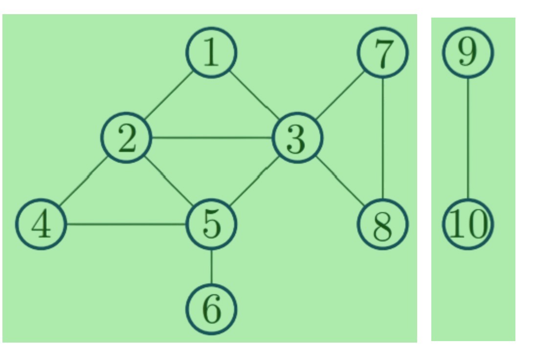
- The connected component of u, con(u), is the set of all vertices connected to u.
- In undirected graphs, connectivity is a refexive, symmetric, and transitive relation. Connected components are the equivalence classes.
- Graph is connected if there is only one connected component.In undirected graphs, connectivity is a refexive, symmetric, and transitive relation. Connected components are the equivalence classes.
- Graph is connected if there is only one connected component. Example:
|
|
|
Basic Graph Search in Undirected Graphs:
| Given G = (V,E) and vertex u $\in$ V. Let n = | V | . Then: |
Explore(G,u):
  Visited[1 . . n] = FALSE
  //ToExplore, S: Lists
  Add u to ToExplore and to S
  Visited[u] = TRUE
  while (ToExplore is non-empty) do
    Remove node x from ToExplore
    for each edge xy in Adj(x) do
      if (Visited[y] = FALSE)
        Visited[y] = TRUE
        Add y to ToExplore
        Add y to S
  Output S
Running time : O(n+m)
- Special cases :
- Breadth First Search (BFS): use queue data structure to implementing the list.
- Depth First Search (DFS): use stack data structure to implement the list.
- Search tree: One can create a natural search tree T rooted at u during search.
Explore(G,u):
array Visited[1..n]
Initialize: Visited[i] = FALSE for i = 1,..., n
List: ToExplore, S
Add u to ToExplore and to S, Visited[u] = TRUE
Make tree T with root as u
while (ToExplore is non-empty) do
  Remove node x from ToExplore
  for each edge (x, y) in Adj(x) do
    if (Visited[y] = FALSE)
      Visited[y] = TRUE
      Add y to ToExplore
      Add y to S
      Add y to T with x as its parent
Output S
II. Directed graphs
Definition
- A directed graph G = (V, E) consists of
- set of vertices/nodes V and
- a set of edges/arcs E \subseteq V x V.
- An edge is an ordered pair of vertices. (u, v) diferent from (v, u).
- Examples:
- Road networks with one-way streets.
- Web-link graph: vertices are web-pages and there is an edge from page p1 to page p2 if p1 has a link to p2.
- Web graphs used by Google with PageRank algorithm to rank pages.
- Dependency graphs in variety of applications: link from x to y if y depends on x. Make fles for compiling programs.
- Program Analysis: functions/procedures are vertices and there is an edge from x to y if x calls y.
Representation
Graph G = (V, E) with n vertices and m edges:
- Adjacency Matrix: n x n asymmetric matrix A. A[u, v] = 1 if (u, v) $\in$ E and A[u, v] = 0 if (u, v) $\notin$ E. A[u, v] is not same as A[v, u].
- Adjacency Lists: for each node u, Out(u) (also referred to as Adj(u)) and In(u) store out-going edges and in-coming edges from u.
|
|
Directed Connectivity
Given a graph G = (V, E):
- A (directed) path is a sequence of distinct vertices $v_1$ , $v_2$ ,…, $v_k$ such that ($v_i$, $v_{i+1}$) $\in$ E for 1 $\le$ i $\le$ k-1. The length of the path is k-1 and the path is from $v_1$ to $v_k$. By convention, a single node u is a path of length 0.
- A cycle is a sequence of distinct vertices $v_1$ , $v_2$ ,…, $v_k$ such that ($v_i$, $v_{i+1}$) $\in$ E for 1 $\le$ i $\le$ k-1 and ($v_k$, $v_1$) $\in$ E. By convention, a single node u is not a cycle.
- A vertex u can reach v if there is a path from u to v. Alternatively v can be reached from u
- Let rch(u) be the set of all vertices reachable from u.
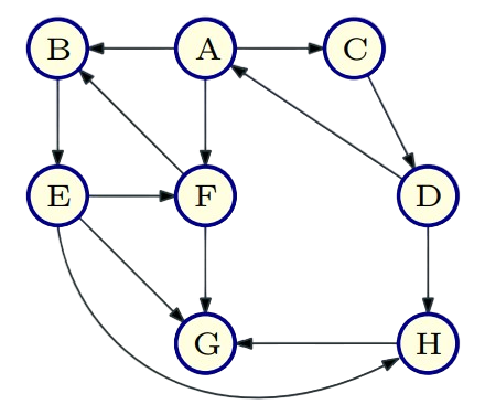
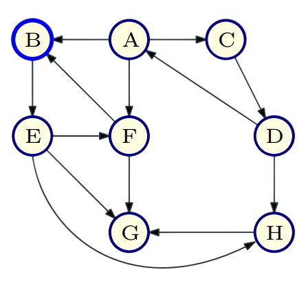
Example of Asymmetricity: D can reach B but B cannot reach D.
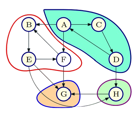
Strong Connected Components
- Defnition: Given a directed graph G, u is strongly connected to v if u can reach v and v can reach u. In other words v $\in$ rch(u) and u $\in$ rch(v).
- Define relation C where uCv if u is (strongly) connected to v.
- Proposition: C is an equivalence relation, that is refexive, symmetric and transitive.
- Equivalence classes of C: strong connected components of G. They partition the vertices of G.
- SCC(u): strongly connected component containing u.
|
|
|
|
Basic Graph Search in Directed Graphs
Given G = (V,E) and vertex u $\in$ V. Let n = |V|. Then:
Explore(G,u):
  array Visited[1..n]
  Initialize: Set Visited[i] = FALSE for 1 <= i <= n
  List: ToExplore, S
  Add u to ToExplore and to S, Visited[u] = TRUE
  Make tree T with root as u
  while (ToExplore is non-empty) do
    Remove node x from ToExplore
    for each edge (x, y) in Adj(x) do
      if (Visited[y] = FALSE)
        Visited[y] = TRUE
        Add y to ToExplore
        Add y to S
        Add y to T with edge (x, y)
  Output S
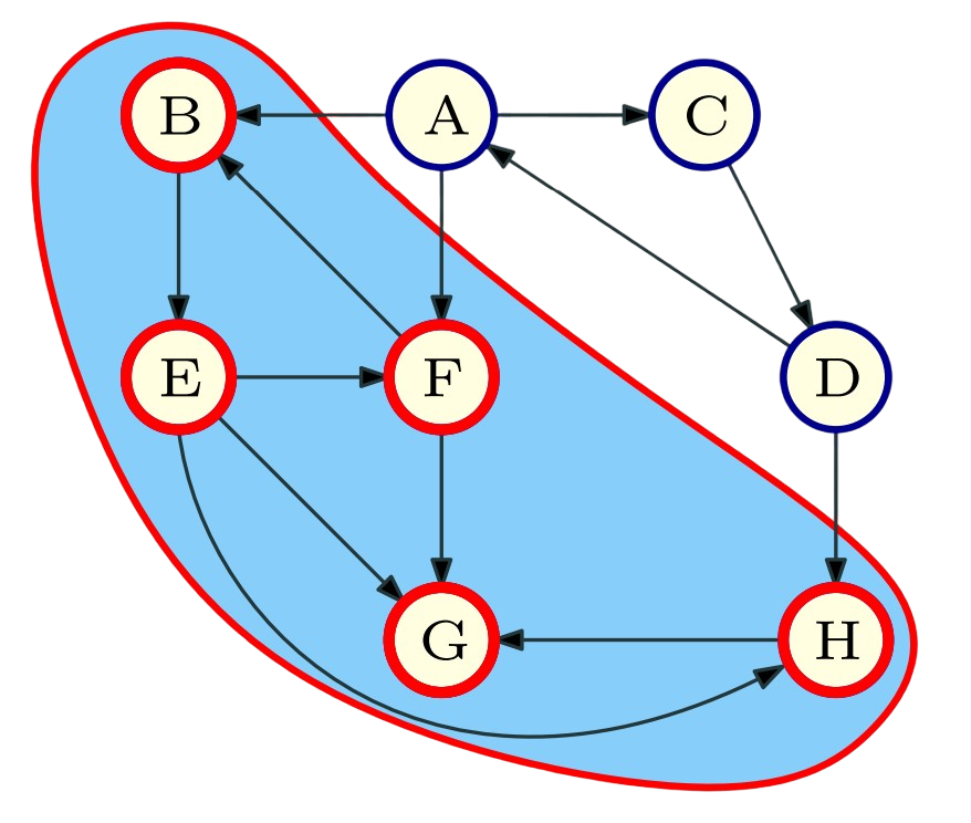
Example - rch(B) :
|
|
|
Basic Graph Search Properties
- Proposition : Explore(G, u) terminates with S = rch(u).
- Proof Sketch.
- Once Visited[i] is set to TRUE it never changes. Hence a node is added only once to ToExplore. Thus algorithm terminates in at most n iterations of while loop.
- By induction on iterations, can show v ∈ S ⇒ v ∈ rch(u)
- Since each node v ∈ S was in ToExplore and was explored, no edges in G leave S. Hence no node in V − S is in rch(u).
- Caveat: In directed graphs edges can enter S.
- Thus S = rch(u) at termination
Relevent LeetCode Practice (by Tristan Yang)
- LeetCode 323 — Number of Connected Components in an Undirected Graph (Medium)
- Relevance: Directly matches the task of finding all connected components in an undirected graph using adjacency lists.
- ECE 374 Process: Build the graph from the given edges, then run a DFS or BFS from each unvisited node, marking all reachable nodes as visited and counting each start as a new component. Runs in $O(n+m)$ for n nodes and m edges.
- Resource: CP-Algorithms tutorial on Depth-First Search (for component counting).
- Takeaway: The basic graph “Explore” pattern (DFS/BFS) can identify components — essentially just repeated graph searches for each component.
- LeetCode 200 — Number of Islands (Medium)
- Relevance: Same connected components idea but on a grid (implicit graph). It reinforces how we model problems as graphs.
- ECE 374 Process: Treat each cell containing ‘1’ as a vertex, with edges connecting adjacent (up/down/left/right) land cells. Then perform DFS/BFS “flood fill” from each unvisited land cell, marking the entire island as visited.
- Resource: NeetCode video on Number of Islands.
- Takeaway: Modeling matters — once you recognize a grid of land/water as a graph, the same search algorithms solve it just like any other component-finding problem.
- LeetCode 785 — Is Graph Bipartite? (Medium)
- Relevance: Classic application of BFS/DFS with 2-coloring (checking bipartiteness via parity of levels).
- ECE 374 Process: Use BFS or DFS to attempt to color the graph with two colors (e.g. +1/-1). Start at any node, color it, then color neighbors with the opposite color. If you ever find an edge connecting two nodes of the same color, the graph isn’t bipartite. Make sure to restart the search for disconnected components.
- Resource: VisuAlgo visualizer – BFS Graph Traversal (demonstrates layering which underpins bipartite check).
- Takeaway: A layered BFS naturally assigns alternating “parity” to levels, which can be used to test bipartiteness (no odd-length cycles present).
- LeetCode 207 — Course Schedule (Medium)
- Relevance: Introduces directed graph reachability and cycle detection, which is a precursor to strongly connected components and topological sorting.
- ECE 374 Process: Build a directed graph of course prerequisites. Then either: (a) perform DFS with 3-color marking (white/gray/black) to detect a back-edge (cycle) if one is found; or (b) perform Kahn’s algorithm (BFS using an in-degree=0 queue) to attempt a topological sort and see if you can pop all nodes. If a cycle exists, you won’t be able to complete all courses.
- Resource: CP-Algorithms article on Topological Sorting.
- Takeaway: Two approaches to detect cycles in directed graphs: DFS (find back-edges via a recursion stack) or BFS (Kahn’s algorithm) — both will indicate if the graph is acyclic or not.
Supplemental Problems
-
LeetCode 133 — Clone Graph
Graph traversal with DFS/BFS and a hash map to copy nodes; good for practicing graph search and handling visited nodes while cloning. -
LeetCode 1971 — Find if Path Exists in Graph
Pure reachability query; simple BFS/DFS or Union-Find to check if two nodes are connected. A warm-up for comparing graph search with union-find methods. -
LeetCode 733 — Flood Fill
Grid DFS/BFS basics; careful about boundary conditions and marking visited (or using the image itself by recoloring). -
LeetCode 994 — Rotting Oranges
Multi-source BFS: start from all initially rotten oranges (multiple sources in the queue) and BFS to compute the minimum minutes for all oranges to rot (layer by layer spread). -
LeetCode 286 — Walls and Gates
Another multi-source BFS: begin from all gates and fill distances to the nearest gate for every room. Shows a reverse-thinking approach (from multiple sources outwards). -
LeetCode 417 — Pacific Atlantic Water Flow
Reverse-reachability on a grid: perform two DFS/BFS (from Pacific coast and from Atlantic coast) to mark cells reachable from each ocean, then intersect the results. Highlights thinking “backwards” from destinations. -
LeetCode 261 — Graph Valid Tree
Check if an undirected graph is a single connected component with no cycles (n nodes, n-1 edges). Can be solved via DFS/BFS (ensure connectivity and no cycle) or via Union-Find (detect cycle and count components). -
LeetCode 310 — Minimum Height Trees
Finds tree centers by repeatedly trimming leaves (like a reverse BFS from all leaves simultaneously). Illustrates a creative application of BFS to find the “middle” of a tree.
Additional Resources
- Textbooks
- Erickson, Jeff. Algorithms
- Skiena, Steven. The Algorithms Design Manual
- Chapter 7.5 - Traversing a Graph
- Sedgewick, Robert and Wayne, Kevin. Algorithms (Forth Edition)
- Chapter 4 - Graphs
- Cormen, Thomas, et al. Algorithms (Forth Edition)
- Chapter 20 - Elementary Graph Algorithms
- Sariel’s Lecture 15
