Lecture 16 - Shortest paths I - BFS and Djikstra

Breadth First Search Algorithm

Breadth First Search (BFS) is a graph traversal algorithm that visits all the vertices of a graph in breadth-first order, i.e., it visits all the vertices at distance 1 from the starting vertex, then all the vertices at distance 2, and so on.

BFS is implemented using a queue data structure, which stores the vertices in the order they are visited. The algorithm starts at a specified vertex, marks it as visited, and adds it to the queue. Then it dequeues the first vertex from the queue, visits all its unvisited neighbors, marks them as visited, and adds them to the queue. This process continues until the queue is empty.

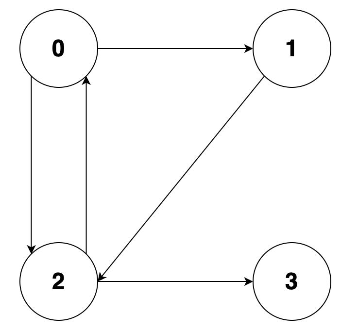
In the above graph, if we start at Node with value 2, the BFS would result in two traversals: (2, 3, 0, 1) or (2, 0, 3, 1).

Time Complexity

The time complexity of BFS is O(|V|+|E|), where |V| is the number of vertices and |E| is the number of edges in the graph. This is because each vertex and edge is visited at most once.

Dijkstra’s Algorithm for Shortest Path

Dijkstra’s algorithm is a graph traversal algorithm that is used to find the shortest path between a starting vertex and all other vertices in a weighted graph. The algorithm maintains a set of visited vertices and a set of unvisited vertices, and it iteratively selects the unvisited vertex with the smallest distance from the starting vertex and visits all its neighboring vertices.

The algorithm works as follows:

1. Initialize the distance of the starting vertex to 0, and the distance of all other vertices to infinity. Mark all vertices as unvisited.
2. Select the unvisited vertex with the smallest distance from the starting vertex, and mark it as visited.
3. For each neighboring vertex that is still unvisited, calculate its tentative distance from the starting vertex by adding the weight of the edge between the two vertices to the distance of the current vertex. If this tentative distance is smaller than the current distance of the neighboring vertex, update its distance to the tentative distance.
4. Repeat steps 2 and 3 until all vertices have been visited, or until the destination vertex (if specified) has been visited.

At the end of the algorithm, the shortest distance from the starting vertex to all other vertices in the graph will have been calculated.

Example:

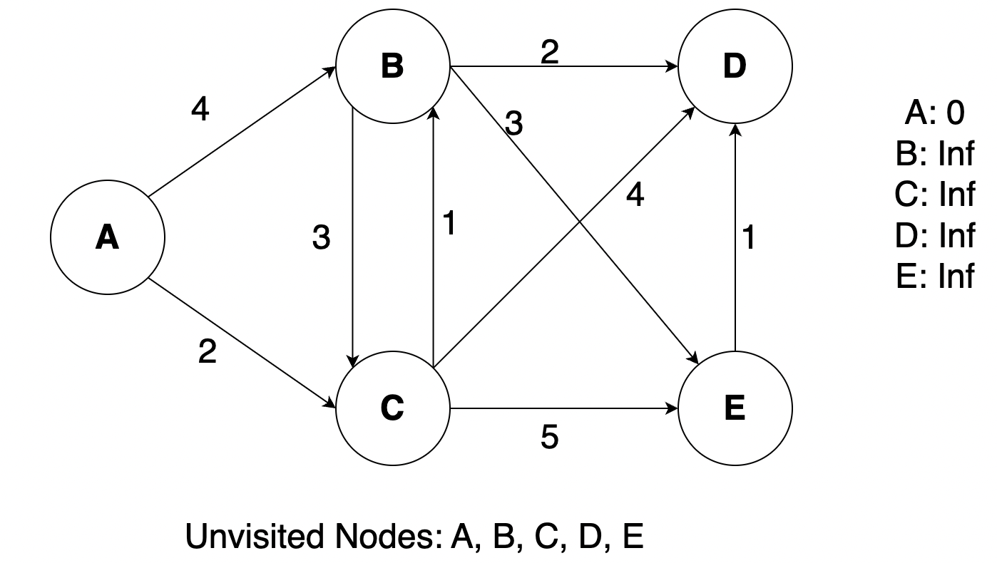
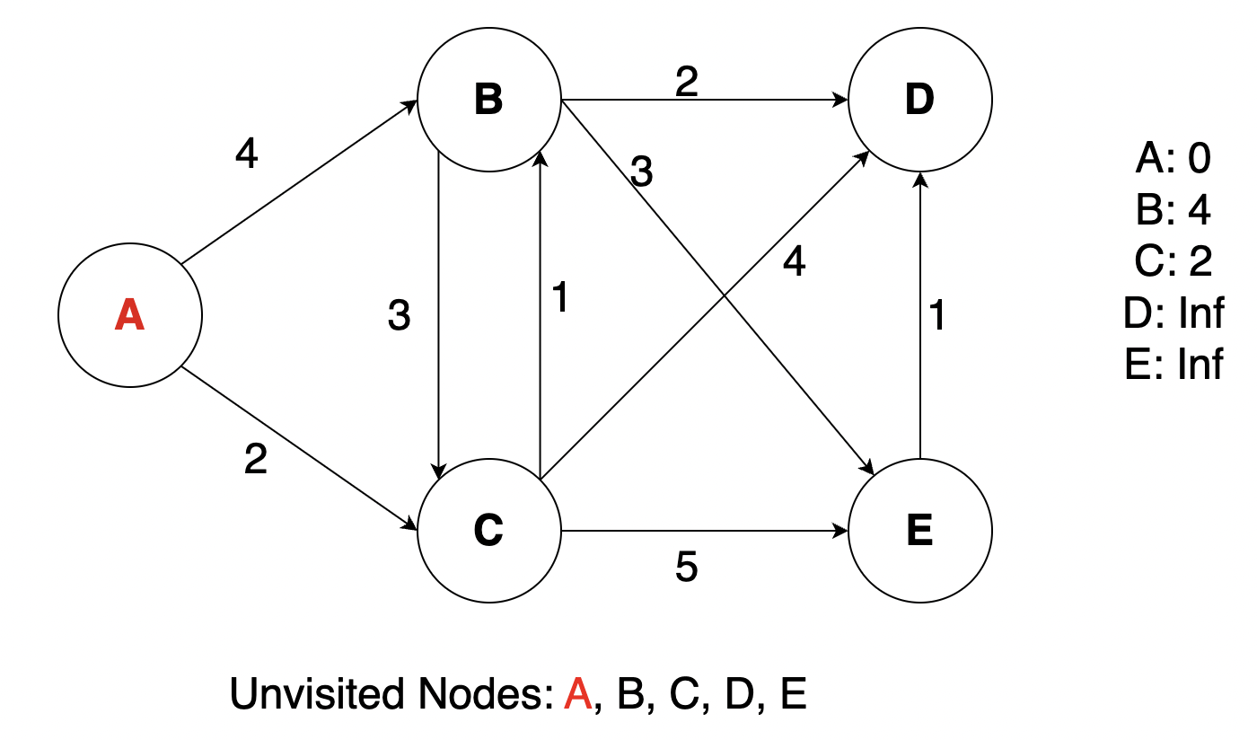
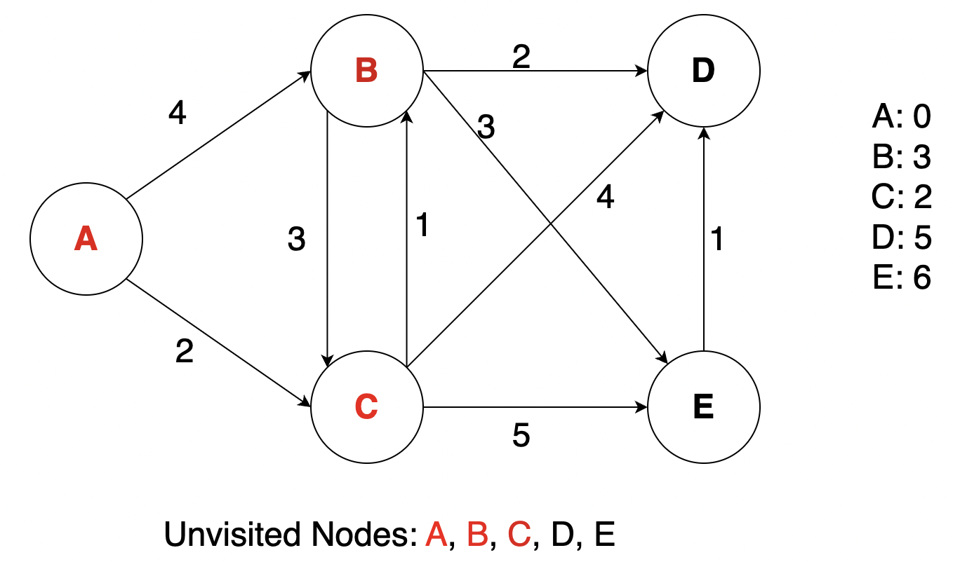
We will find the min distance from A to all other nodes in the graph. Initially the distance will be mapped as Infinity (inf) for all nodes other than A and we will also maintain an unvisited Array at the bottom. First we will mark A as visited and then update the distance maps based on the nodes that A has edges to.

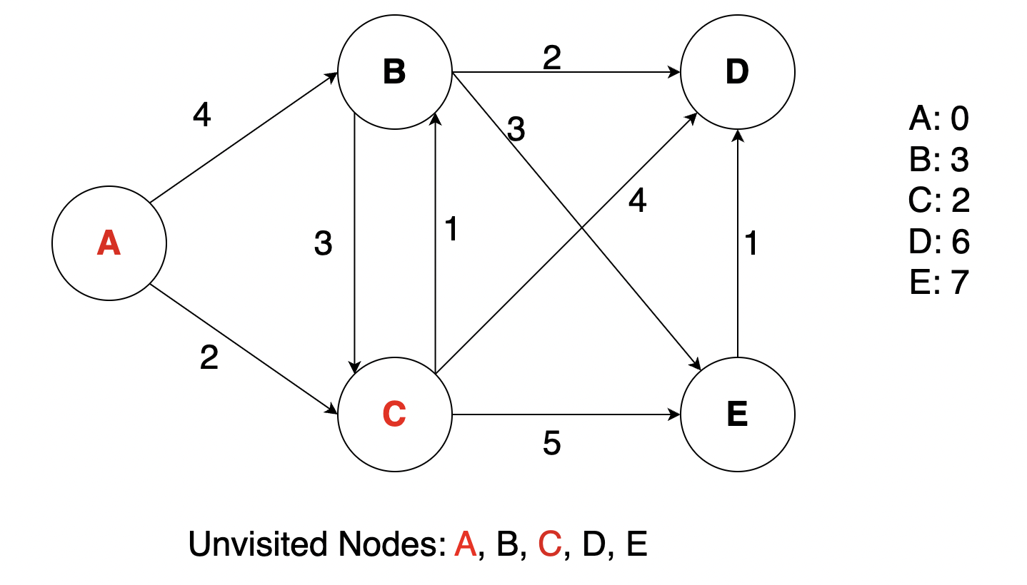
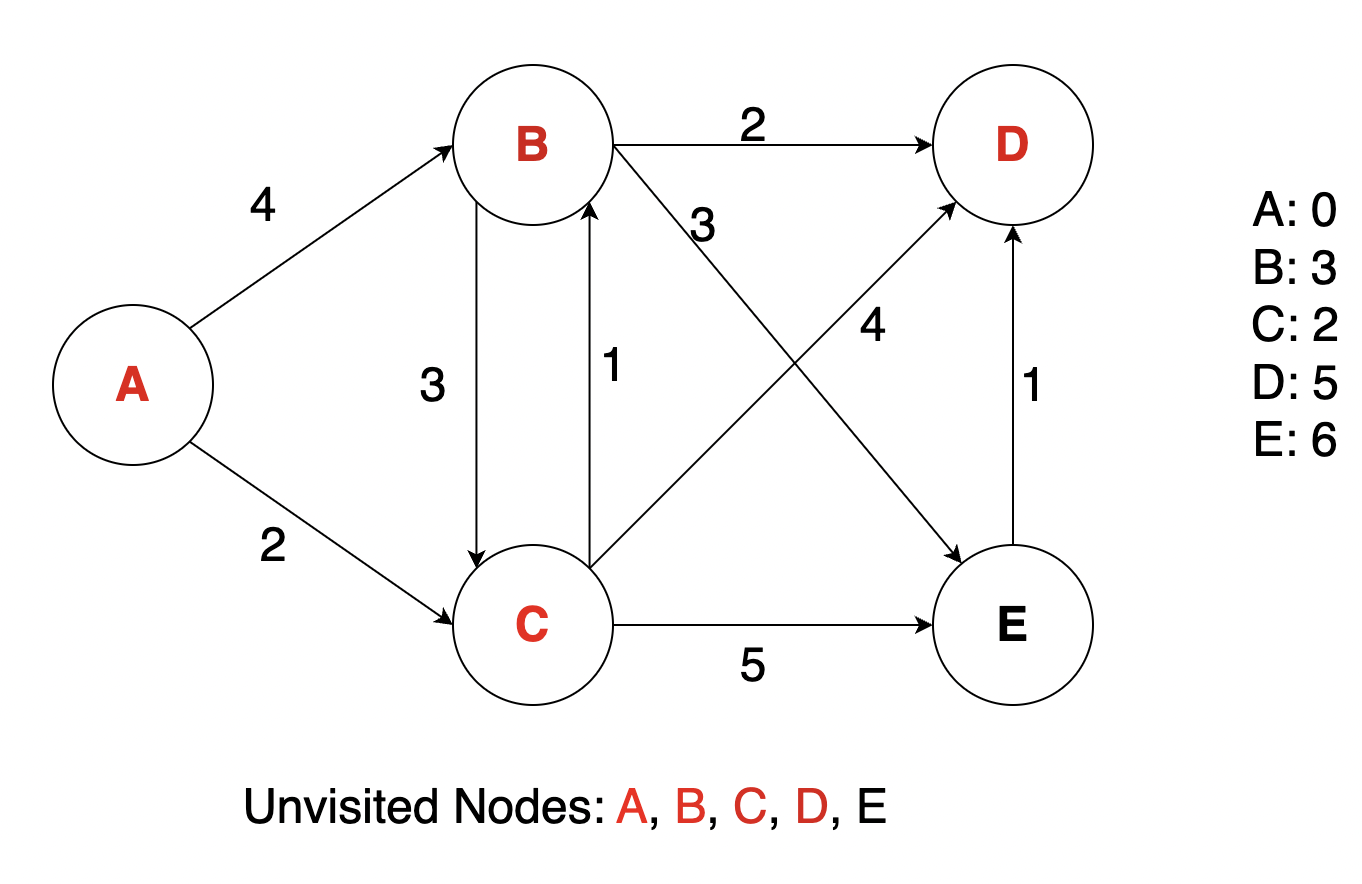
We see that C is the next unvisited node with shortest distance, so we will now mark C as visited and update the distance map.

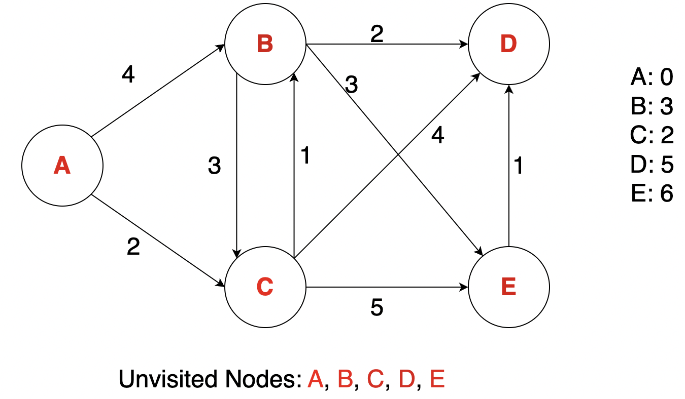
Next we do similar steps with B, D, E

Time Complexity

Dijkstra’s Algorithm with Priority Queue

Dijkstra’s algorithm can be implemented using a priority queue data structure to efficiently select the unvisited vertex with the smallest distance from the starting vertex.

The algorithm works as follows:

1. Initialize the distance of the starting vertex to 0, and the distance of all other vertices to infinity. Insert all vertices into the priority queue.
2. While the priority queue is not empty, remove the vertex with the smallest distance from the starting vertex (the root of the priority queue).
3. If the removed vertex is the destination vertex (if specified), terminate the algorithm and return the shortest distance.
4. For each neighboring vertex of the removed vertex that is still in the priority queue, calculate its tentative distance from the starting vertex by adding the weight of the edge between the two vertices to the distance of the removed vertex. If this tentative distance is smaller than the current distance of the neighboring vertex, update its distance to the tentative distance and update its position in the priority queue accordingly.
5. Repeat steps 2-4 until the destination vertex has been visited, or until the priority queue is empty.

Time Complexity

Relevent LeetCode Practice (by Tristan Yang)

1. LeetCode 743 — Network Delay Time (Medium)
   • Relevance: The canonical single-source shortest path problem on a directed weighted graph (with all edges having non-negative weight).
   • ECE 374 Process: Use Dijkstra’s algorithm starting from the given source node k. Maintain a min-heap of (distance, node) pairs; repeatedly extract the nearest unprocessed node and relax its outgoing edges. After processing, the answer is the maximum distance to any node (or report -1 if some node is unreachable).
   • Resource: NeetCode video on Network Delay Time.
   • Takeaway: Dijkstra explores nodes in increasing order of tentative distance, ensuring that the first time you finalize a node’s distance, you have found the shortest path to it.
2. LeetCode 787 — Cheapest Flights Within K Stops (Medium)
   • Relevance: A shortest path problem with an added constraint on the number of edges (stops). This can be approached by modified BFS/DP or an expanded state-space Dijkstra.
   • ECE 374 Process: Three approaches: DP/Bellman-Ford for at most K+1 edges (K relaxations). BFS in layers (each layer represents one more stop), with cost pruning to avoid superfluous exploration. Dijkstra on an expanded state space (state = node + stops used), ignoring or not exploring paths that exceed K stops.
   • Resource: NeetCode video on Cheapest Flights Within K Stops.
   • Takeaway: You can encode the “at most K stops” constraint by augmenting the state with the count of stops, effectively adding a layer dimension to the search (and requiring careful handling in the algorithm).
3. LeetCode 1368 — Minimum Cost to Make at Least One Valid Path in a Grid (Hard)
   • Relevance: A classic 0-1 BFS problem (edge weights are only 0 or 1). It exemplifies when a deque-based BFS can outperform a generic priority queue approach.
   • ECE 374 Process: Model the grid moves as a graph where moving in the preferred direction of an arrow has cost 0, and changing direction (going against the arrow) costs 1. Use a deque for 0-1 BFS: push neighbors reached with 0 cost to the front, and neighbors reached with cost 1 to the back. The first time you reach the target cell, you have the minimum cost.
   • Resource: CP-Algorithms description of 0-1 BFS.
   • Takeaway: 0-1 BFS is an optimization of Dijkstra when edge weights are only 0 or 1. It avoids the overhead of heap operations by using a deque to maintain nodes to explore.
4. LeetCode 1976 — Number of Ways to Arrive at Destination (Medium)
   • Relevance: Asks for counting the number of shortest paths, not just computing one distance — a common extension of shortest path problems.
   • ECE 374 Process: First, run Dijkstra to find the shortest distance to each node from the start. Then, you can count paths either during the Dijkstra (maintaining a count array and updating it whenever a shortest distance is found or matched) or after: perform a DP in order of increasing distance. For each edge $(u,v)$, if dist[u] + w == dist[v], add the number of ways to reach $u$ to the number of ways to reach $v$. Remember to mod the results if required.
   • Resource: NeetCode video on Number of Ways to Arrive at Destination.
   • Takeaway: Combine Dijkstra with a counting mechanism: when a new shorter path to a node is found, reset the count; when an equally short path is found, increment the count. This yields the total number of distinct shortest paths.

Supplemental Problems

• LeetCode 1786 — Number of Restricted Paths From First to Last Node
  Variation on path counting: first run Dijkstra from the last node to get distances to every node. Then count, via DFS or DP, how many paths from 1 to n are “restricted” (each step going to a node with smaller distance to n). This forms a DAG by distance.

• LeetCode 1129 — Shortest Path with Alternating Colors
  Graph with red and blue edges. Use BFS on a state space where state includes the current node and the color of the edge just taken. Ensure that you alternate colors as you traverse.

• LeetCode 847 — Shortest Path Visiting All Nodes
  A BFS on the state = (node, bitmask_of_visited_nodes). This is essentially the Traveling Salesman Problem on a small graph, solved by BFS since $2^n$ states with n up to maybe 12 or so.

• LeetCode 505 — The Maze II
  A shortest distance problem in a grid where you “roll” a ball until it hits a wall. Use Dijkstra because each move covers potentially many cells and you accumulate distance. Similar to a standard grid BFS but with different transition rules.

• LeetCode 499 — The Maze III
  Extension of Maze II: find not only the shortest distance for the ball to stop at the hole, but also the lexicographically smallest path string among shortest paths. This can be handled by augmenting state with the path or by custom comparison in the priority queue (distance first, then path string).

• LeetCode 126 — Word Ladder II
  Find all shortest transformation sequences, not just one. Use BFS from the begin word to find the distance to each word (like Word Ladder I), then build a predecessor graph of word transitions. Finally, use backtracking (DFS) from the end word to construct all sequences that achieve that shortest distance.

Additional Resources

• Textbooks
  • Erickson, Jeff. Algorithms
    • Chapter 8 - Shortest Paths
    • Chapter 9 - All-Pairs Shortest Paths
  • Skiena, Steven. The Algorithms Design Manual
    • Chapter 7.6 - Breadth-First Search
    • Chapter 8.3 - Shortest Path
  • Sedgewick, Robert and Wayne, Kevin. Algorithms (Forth Edition)
    • Chapter 4.1 - Breadth-First Search
    • Chapter 4.4 - Shortest Paths
  • Cormen, Thomas, et al. Algorithms (Forth Edition)
    • Chapter 20.2 - Breadth-First Search
    • Chapter 22.1 - The Bellman-Ford Algorithm
• Sariel’s Lecture 17